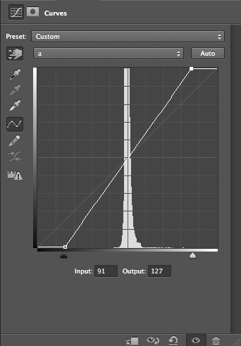

a Curve Before

a Curve After Adjustment

b Curve Before

b Curve After Adjustment
Where we last left off on our Lab adventure we’d described a colorspace that could enhance and separate colors with both the a and b channels. These channels respond wildly to increased contrast, in ways that border on miraculous. Colors increase in saturation, separation, and definition. It is the most basic and fundamental move in the Lab-editing arsenal.
Although that can be accomplished a number of ways, the classic and most flexible approach is to apply a Curve adjustment layer in Photoshop. The Curve adjustment (in general) is highly unappreciated. It seems that software developers are constantly creating workarounds and cute sliders to dumb-down this most elegant tool or to avoid it entirely. In spite of this, it remains relevant and powerful—yet many people seem to avoid it. At its essence, a Curve adjustment is a graphical, transfer function. Image data go into the adjustment and come on altered depending upon how we bend and shape the curve. The adjustment is clean and simple but endlessly fascinating in its variation.
I can understand the aversion to Curves. I was introduced to tonal curves many years ago during my undergraduate work at the Rochester Institute of Technology. We’d expose sheets of film in sensitometers and plot the resulting densities on graph paper. I hated everything about the entire process and cursed every data point I ever plotted. Little did I know that this numbing exercise would eventually give me an intrinsic understanding of today’s application of the tone-reproduction curve. And that’s the thing about the Curve adjustment layer. It takes practice and lot more of it than you’d suspect.
The flexibility of Curves adjustment layer is demonstrated in its use with our basic Lab move, which I will now describe. We apply the layer and steepen the curves of the a and b channels in a straight-line and equal fashion to both the top and bottom of the each curve. We keep the middle of the curve intersected at the midpoint of the graph. Otherwise we’ll introduce a colorcast to the image. Later on, we might exploit this phenomenon to correct an undesirable cast but, for now, we’ll avoid such adventures. The curves are simply steepened and we then look at the result. If we want more or less effect, we either lower or raise the angle accordingly. After awhile we can start to predict the results with uncanny accuracy. That’s where the practice comes in.
This gets to be so much fun that we might start to enhance images to within an inch of their life. This should be avoided. The imaging world is plagued with over-saturated, over-processed and downright ugly images. I’d hate to see the power of Lab be abused by its overuse. Be careful with this. You don’t want to blow out colors and drive them out-of-gamut (so that they can’t be reproduced nor do they retain any details). Images should not look like bad acid trips. Nor should they glow like a science-fiction film from the beginning of the Atomic Age. Restraint is essential here. And this is why Curve adjustments are so crucial. They give us the control and finesse (along with other tools like layer masks, blending modes, and advanced blending options, but those tools are best left for another discussion on another day). For now, just be careful with the amount of adjustment you apply and don’t use this technique on images that already contain lots of bright, saturated colors.
This entire technique was developed by Dan Margulis. If you want to really learn from the master, you should read his book, Photoshop LAB Color: The Canyon Conundrum and Other Adventures in the Most Powerful Colorspace.
Technique
1. Convert image to Lab mode. The easiest way to convert your image to Lab mode is to go to the pulldown menu in Photoshop and choose Image>Mode>Lab Color. A more unerring way to convert images back-and-forth between Lab and RGB is to choose Edit>Convert to Profile…. This will give you more options for color spaces which is essential particularly when converting from Lab to RGB or CMYK. For this part of the technique we'll simply choose for our destination space, "Lab Color."
2. Add a Curve adjustment layer to the top of the layer stack. You can do this by clicking on the Curves icon in the Adjustments panel or by clicking on the little Zen-like half-black, half-white circle on the bottom of the Layers panel.
3. Steepen the a and b curves. Select the a-channel curve and drag the top and bottom points of the curve in equal amounts to steepen the curve. Do not allow the curve to deviate from a straight line and keep the center of the curve in the exact middle of the curve’s grid. Do the same thing now with the b-channel curve.
4. Review the image and season to taste. The image might look great or might need more or less of this adjustment. Either steepen the curves more or do the opposite. If one particular color needs more or less of an adjustment you might change either the a or b curve independently of the other (i.e., if the sky needs more blue accentuation try steepening the b channel more than the a channel curve. Yellow-to-blue colors are defined by the b channel).